What is an image

An image can be thought of as a grid of numbers, like a matrix. The grid consists of rows (representing the image’s height) and columns (representing the width), where each value in the matrix corresponds to a single pixel. The pixel value determines the brightness of that spot in the image:

• A larger value means a brighter pixel.

• A smaller value means a darker pixel.

Pixel values of most types of images are often represented as 8-bit unsigned integers ranging from 0 to 255:

• 0 corresponds to black (the darkest pixel).

• 255 corresponds to white (the brightest pixel).

Note

Most scientific images, such as those from fluorescence microscopes, use higher-bit integers and therefore capture a wider range of values. For example, many fluorescence microscopes produce 16-bit images, which can range from 0 to 65,535.

Let’s consider an example of three 8 × 8 matrices, where each matrix contains different pixel values and visualize them as images.

import numpy as np
import matplotlib.pyplot as plt


matrix_1 = np.array([[  0,   0,   0,   0,   0,   0,   0,   0],
                     [  0,   0,   0,  63,  63,   0,   0,   0],
                     [  0,   0,  63, 127, 127,  63,   0,   0],
                     [  0,  63, 127, 255, 255, 127,  63,   0],
                     [  0,  63, 127, 255, 255, 127,  63,   0],
                     [  0,   0,  63, 127, 127,  63,   0,   0],
                     [  0,   0,   0,  63,  63,   0,   0,   0],
                     [  0,   0,   0,   0,   0,   0,   0,   0]])

matrix_2 = np.array([[  0,   0,   0,   0,   0,   0,   0,   0],
                     [  0,   0,   0,   0,  63,  63,   0,   0],
                     [  0,   0,   0,  63, 127, 127,  63,   0],
                     [  0,   0,  63, 127, 255, 255, 127,  63],
                     [  0,   0,  63, 127, 255, 255, 127,  63],
                     [  0,   0,   0,  63, 127, 127,  63,   0],
                     [  0,   0,   0,   0,  63,  63,   0,   0],
                     [  0,   0,   0,   0,   0,   0,   0,   0]])

matrix_3 = np.array([[  0,   0,   0,   0,   0,   0,   0,   0],
                     [  0,   0,   0,   0,   0,   0,   0,   0],
                     [  0,   0,   0,  63,  63,   0,   0,   0],
                     [  0,   0,  63, 127, 127,  63,   0,   0],
                     [  0,  63, 127, 255, 255, 127,  63,   0],
                     [  0,  63, 127, 255, 255, 127,  63,   0],
                     [  0,   0,  63, 127, 127,  63,   0,   0],
                     [  0,   0,   0,  63,  63,   0,   0,   0]])


plt.figure(figsize=(11,3))

plt.subplot(131)
plt.title('matrix 1')
plt.imshow(matrix_1, cmap='gray')

plt.subplot(132)
plt.title('matrix 2')
plt.imshow(matrix_2, cmap='gray')

plt.subplot(133)
plt.title('matrix 3')
plt.imshow(matrix_3, cmap='gray')

plt.show()

When visualized, these matrices appear as grayscale images and the pixels with higher values appear brighter.

Colored Images

While grayscale images are represented by a 2D matrix (height × width), colored images are represented by a 3D matrix with the size (height × width × 3).

Here, the 3 channels represent the three primary colors: Red (R), Green (G), Blue (B). Each pixel in an RGB image has three values (one for each channel).

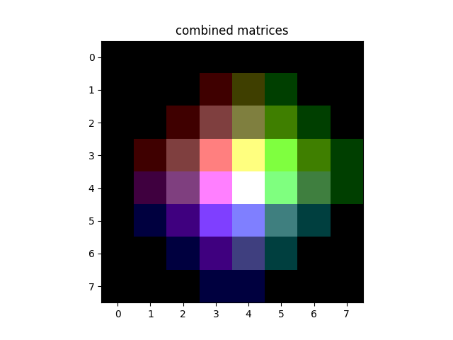
For example, we can stack the three 8 × 8 matrices, matrix 1 for Red, 2 for Green, and 3 for Blue, results in an 8 × 8 × 3 matrix and visualize it as a colored image.

combined_matrices = np.dstack([matrix_1,
                               matrix_2,
                               matrix_3])

print(combined_matrices.shape)

plt.figure()
plt.title('combined matrices')
plt.imshow(combined_matrices)
plt.show()

(8, 8, 3)

As we can see:

• When a pixel has R, G, and B values of 255 (e.g., at position (4,4)), the pixel appears white.

• If the Red channel value is high while the others are low, the color becomes redder.

• Similarly, higher values in the Blue or Green channels make the pixel appear bluer or greener, respectively.

By adjusting the values in these three channels, we can represent any color in an image.