Extracting Information (Masking)

Arguably (because this is my personal opinion), the most common application of binary image is to extract information.

Basic Concept

In this context, a binary image is often referred to as a binary mask because it is used to mask or filter specific regions of interest. This process is known as image masking.

To demonstrate how this works, will use 8x8 grayscale and binary images.

import numpy as np
import matplotlib.pyplot as plt
import matplotlib.patheffects as path_effects

binary_image = np.array([[0, 0, 0, 0, 0, 0, 0, 0],
                         [0, 0, 0, 1, 1, 0, 0, 0],
                         [0, 0, 1, 1, 1, 1, 0, 0],
                         [0, 1, 1, 1, 1, 1, 1, 0],
                         [0, 1, 1, 1, 1, 1, 1, 0],
                         [0, 0, 1, 1, 1, 1, 0, 0],
                         [0, 0, 0, 1, 1, 0, 0, 0],
                         [0, 0, 0, 0, 0, 0, 0, 0]])

grayscale_image = np.array([[0. , 0. , 0. , 0. , 0. , 0. , 0. , 0. ],
                            [0. , 0. , 0. , 0.1, 0.2, 0.1, 0. , 0. ],
                            [0. , 0. , 0.1, 0.3, 0.4, 0.2, 0.1, 0. ],
                            [0. , 0.1, 0.3, 0.7, 0.8, 0.6, 0.2, 0.1],
                            [0. , 0.2, 0.4, 0.8, 1. , 0.7, 0.3, 0.1],
                            [0. , 0.1, 0.2, 0.6, 0.7, 0.4, 0.2, 0. ],
                            [0. , 0. , 0.1, 0.2, 0.3, 0.2, 0. , 0. ],
                            [0. , 0. , 0. , 0.1, 0.1, 0. , 0. , 0. ]])

# Function to display image with mask or pixel values
def display_image(ax, img, title, mask=None, show_value=False):
    if mask is not None:
        masked_img = np.where(mask, img, np.nan)
    else:
        masked_img = img

    ax.imshow(masked_img, cmap='gray', vmin=img.min(), vmax=img.max())
    ax.set_title(title)
    ax.axis("off")

    if show_value:
        for row in range(img.shape[0]):
            for col in range(img.shape[1]):
                if mask is None or mask[row, col]:
                    text = ax.text(col, row, img[row, col], ha='center', va='center',
                                   fontsize=12, color='black', fontweight='bold')
                    text.set_path_effects([path_effects.Stroke(linewidth=2, foreground='white'),
                                           path_effects.Normal()])

fig, axes = plt.subplots(1, 3, figsize=(12, 4))
display_image(axes[0], grayscale_image, "Grayscale Image", show_value=True)
display_image(axes[1], binary_image, "Binary mask")
display_image(axes[2], grayscale_image, "Masked Image", mask=binary_image, show_value=True)
plt.tight_layout()
plt.show()

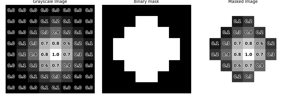
Essentially, we use a binary mask when we want to extract values only from the areas it defines.

In python, using numpy this can simply be done by boolean indexing.

# Extract the value by indexing
masked_value = grayscale_image[binary_image.astype(bool)]

print(masked_value)

[0.1 0.2 0.1 0.3 0.4 0.2 0.1 0.3 0.7 0.8 0.6 0.2 0.2 0.4 0.8 1.  0.7 0.3
 0.2 0.6 0.7 0.4 0.2 0.3]

Practical example

To see this in action, we’ll use use images of protein translocation described in this paper from our lab. The images were kindly provided by the corresponding author.

Context and Objective

These fluorescence images capture the translocation of a protein of interest (POI) from the cytosol to the nucleus. The dataset consists of two channels: one for the POI and one for the nucleus. Let’s apply information extraction to visualize this process.

from tifffile import imread
from skimage.filters import threshold_otsu

POI_ch = imread("images/miRFP670nano_sample.tif")
nucleus_ch = imread("images/mOrange2_sample.tif")

print(POI_ch.shape, nucleus_ch.shape)
# We have 71 frames of 150×185 images

(71, 150, 185) (71, 150, 185)

Extracting Fluorescence from Nucleus

Let’s say we want to know how much POI is located in the nucleus at each time point.

First, we can locate the nucleus by generating a binary mask from the nucleus channel. Then, we extract the fluorescence intensity of the POI using this mask.

To demonstrate this, we can use the images from the first frame.

# The first frame as an example
nucleus_1 = nucleus_ch[0]
POI_1 = POI_ch[0]

# Thresholding to get the mask
th = threshold_otsu(nucleus_1)
nucleus_mask = nucleus_1 > th

# Extract the fluorescence intensity from both channels
POI_fl_1 = POI_1[nucleus_mask]
nucleus_fl_1 = nucleus_1[nucleus_mask]

fig, axes = plt.subplots(1, 4, figsize=(12, 3))
display_image(axes[0], nucleus_mask, "Nucleus Mask")
display_image(axes[1], POI_1, "POI")
display_image(axes[2], POI_1, "POI in nucleus", mask=nucleus_mask)
display_image(axes[3], nucleus_1, "Nucleus fluorescence", mask=nucleus_mask)
plt.tight_layout()
plt.show()

print(f"average fluorescence intensity of POI in nucleus: {POI_fl_1.mean()}")
print(f"average fluorescence intensity of nucleus protein: {nucleus_fl_1.mean()}")

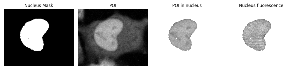
average fluorescence intensity of POI in nucleus: 1032.8508311461067
average fluorescence intensity of nucleus protein: 258.5612423447069

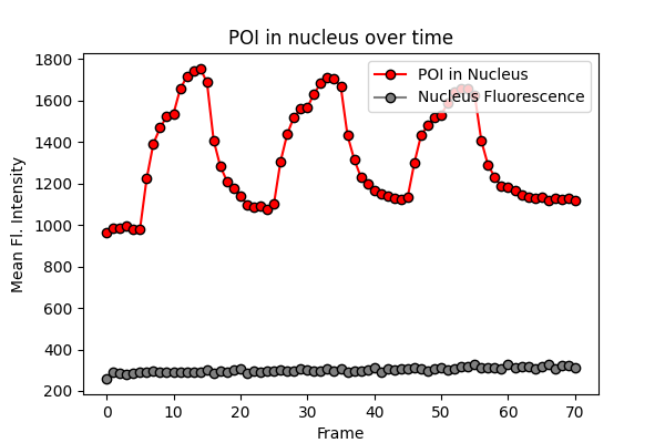
Tracking Fluorescence Changes in Nucleus

Let’s put it together into one function so we can apply the process (thresholding to get the mask -> extract fluorescence intensity) into all the frames.

def extract_fluorescence_intensity(image, mask_function):
    num_frames = image.shape[0]
    mean_intensity = []

    for i in range(num_frames):
        mask = mask_function(image[i])
        masked_values = image[i][mask]
        mean_intensity.append(masked_values.mean())

    return mean_intensity

# Function to get the mask by thresholding
def nucleus_mask_function(frame):
    return frame > threshold_otsu(frame)

# Apply function to all frames
POI_nucleus_intensities = extract_fluorescence_intensity(POI_ch, nucleus_mask_function)
nucleus_intensities = extract_fluorescence_intensity(nucleus_ch, nucleus_mask_function)

# Plotting the mean fluorescence intensity over time

fig, ax = plt.subplots(figsize=(6, 4))
ax.plot(POI_nucleus_intensities, label="POI in Nucleus", marker='o', c='red', mec='k')
ax.plot(nucleus_intensities, label="Nucleus Fluorescence", marker='o', c='gray', mec='k')
ax.set_xlabel("Frame")
ax.set_ylabel("Mean Fl. Intensity")
ax.set_title("POI in nucleus over time")
ax.legend()
plt.show()

Creating Cytosol Mask

Okay, so now we can see the translocation of POI to and from nucleus. But how do we know that it’s from cytosol?

Well, we can get the mean fluorescence intensity from the cytosol and see the correlation. But we don’t have a cytosol channel.

One creative way to do that is by expanding the nucleus mask. Because we know that the cytosol surrounds the nucleus.

from skimage.morphology import binary_dilation, disk

# Expand nucleus mask to define a surrounding region
nucleus_dilate_1 = binary_dilation(nucleus_mask, disk(3))
nucleus_dilate_2 = binary_dilation(nucleus_mask, disk(5))

# Define cytosol region as the ring between two dilations
cytosol_mask = nucleus_dilate_2 ^ nucleus_dilate_1  # Subtract (nucleus_dilate_2 - nucleus_dilate_1) also works in this case

fig, axes = plt.subplots(1, 4, figsize=(12, 3))
display_image(axes[0], nucleus_mask, "Nucleus Mask")
display_image(axes[1], nucleus_dilate_1, "Dilation 1 (A)")
display_image(axes[2], nucleus_dilate_2, "Dilation 2 (B)")
display_image(axes[3], cytosol_mask, "Around Nucleus (A ^ B)")
plt.tight_layout()
plt.show()

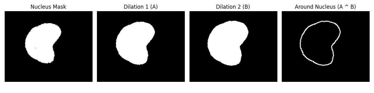
Neat, huh?! This is actually an approach I followed from this paper.

Now, let’s see if this can be used in our case

fig, axes = plt.subplots(1, 3, figsize=(12, 4))
display_image(axes[0], POI_1, "POI")
display_image(axes[1], POI_1, "POI in nucleus", mask=nucleus_mask)
display_image(axes[2], POI_1, "POI around nucleus", mask=cytosol_mask)
plt.tight_layout()
plt.show()

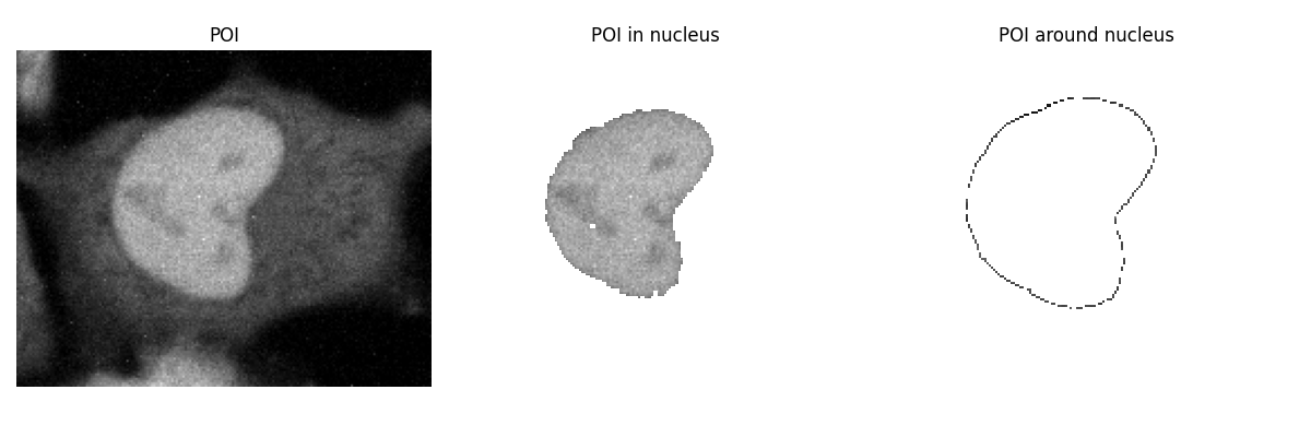
The cytosol(ish) mask also includes a little area outside of the cell, but overall, it looks pretty good!

Comparing Nucleus and Cytosol Fluorescence

Let’s apply this to all frames and compare it to the fluorescence intensity in the nucleus.

# Function to generate cytosol mask
def cytosol_mask_function(frame):
    nucleus_mask = nucleus_mask_function(frame)
    nucleus_dilate_1 = binary_dilation(nucleus_mask, disk(3))
    nucleus_dilate_2 = binary_dilation(nucleus_mask, disk(5))
    return nucleus_dilate_2 ^ nucleus_dilate_1  # Cytosol mask

# Apply function to all frames
POI_cytosol_intensities = extract_fluorescence_intensity(POI_ch, cytosol_mask_function)
cytosol_intensities = extract_fluorescence_intensity(nucleus_ch, cytosol_mask_function)

# Plotting the mean fluorescence intensity of POI in nucleus and cytosol over time

fig, ax1 = plt.subplots(figsize=(6,4))

ax1.plot(POI_nucleus_intensities, label="POI in Nucleus", marker='o', c='red', mec='k')
ax1.set_xlabel("Frame")
ax1.set_ylabel("Mean Fl. Intensity (Nucleus)")
ax1.tick_params(axis='y', labelcolor='red')

ax2 = ax1.twinx()
ax2.plot(POI_cytosol_intensities, label="POI in Cytosol", marker='o', c='blue', mec='k')
ax2.set_ylabel("Mean Fl. Intensity (Cytosol)")
ax2.tick_params(axis='y', labelcolor='blue')

fig.legend(bbox_to_anchor=(1, 1), bbox_transform=ax1.transAxes)
ax1.set_title("POI Fl. Intensity Over Time")
plt.show()

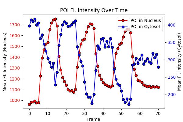
We can clearly see that as the intensity of POI in the nucleus increases, the intensity in the cytosol decreases. Likewise, when the POI intensity in the nucleus decreases, it increases in the cytosol. This indicates that POI translocates between the nucleus and cytosol.

Note

In the paper, the authors calculated the correlation between the two channels (Pearson’s correlation coefficient) to quantify the translocation, instead of calculating the fluorescence intensity. Why do you think that is?